Week 9 - Hands-On Examples

week09
exercise

The R script is available here: link

Goals

  • Know how to process strings in the data
  • Get familiar with the main tidyverse packege for data manipulation and visualisation.

Mini Data Project

Data Import & Exploration

  1. Import the following datasets using the appropriate functions:
  • Yeast gene annotation data: "https://raw.githubusercontent.com/InforBio/IOC/refs/heads/main/ioc_r/exos_data/mart_export.txt.gz", name the data as annot.
  • Gene differential expression analysis (SET1 vs. WT): "https://inforbio.github.io/IOC/ioc_r/exos_data/toy_DEanalysis.csv", name the data as de_res.

What are the dimensions of each dataset?

library(tidyverse)
── Attaching core tidyverse packages ──────────────────────── tidyverse 2.0.0 ──
✔ dplyr     1.1.4     ✔ readr     2.1.5
✔ forcats   1.0.0     ✔ stringr   1.5.1
✔ ggplot2   3.5.1     ✔ tibble    3.2.1
✔ lubridate 1.9.4     ✔ tidyr     1.3.1
✔ purrr     1.0.4     
── Conflicts ────────────────────────────────────────── tidyverse_conflicts() ──
✖ dplyr::filter() masks stats::filter()
✖ dplyr::lag()    masks stats::lag()
ℹ Use the conflicted package (<http://conflicted.r-lib.org/>) to force all conflicts to become errors
annot <- read_csv(
  "https://raw.githubusercontent.com/InforBio/IOC/refs/heads/main/ioc_r/exos_data/mart_export.txt.gz"
)
Rows: 7127 Columns: 9
── Column specification ────────────────────────────────────────────────────────
Delimiter: ","
chr (5): Gene stable ID, Gene type, Gene name, Chromosome/scaffold name, Gen...
dbl (4): Gene % GC content, Transcript count, Gene start (bp), Gene end (bp)

ℹ Use `spec()` to retrieve the full column specification for this data.
ℹ Specify the column types or set `show_col_types = FALSE` to quiet this message.
de_res <- read_csv("https://inforbio.github.io/IOC/ioc_r/exos_data/toy_DEanalysis.csv")
Rows: 45 Columns: 7
── Column specification ────────────────────────────────────────────────────────
Delimiter: ","
chr (1): gene_name
dbl (6): baseMean, log2FoldChange, lfcSE, stat, pvalue, padj

ℹ Use `spec()` to retrieve the full column specification for this data.
ℹ Specify the column types or set `show_col_types = FALSE` to quiet this message.
  1. Which chromosome has the highest number of genes? Which chromosome has the lowest number of genes?
annot |>
  count(`Chromosome/scaffold name`) |>
  arrange(n)
# A tibble: 17 × 2
   `Chromosome/scaffold name`     n
   <chr>                      <int>
 1 Mito                          55
 2 I                            126
 3 VI                           156
 4 III                          202
 5 IX                           259
 6 VIII                         340
 7 V                            356
 8 XI                           369
 9 X                            434
10 XIV                          459
11 II                           478
12 XVI                          545
13 XIII                         549
14 XV                           636
15 VII                          639
16 XII                          639
17 IV                           885
annot |>
  count(`Chromosome/scaffold name`) |>
  arrange(n) |>
  slice(1, n()) # extract the 1st and the last rows
# A tibble: 2 × 2
  `Chromosome/scaffold name`     n
  <chr>                      <int>
1 Mito                          55
2 IV                           885
  1. Among mitochondrial genes, find those where the gene description contains “ATP6” or “ATP8”. Then select and display only the columns: “Gene name” and “Gene description”.
annot |>
  filter(`Chromosome/scaffold name` == "Mito") |>
  filter(str_detect(`Gene description`, "ATP[68]")) |>
  select(`Gene name`, `Gene description`)
# A tibble: 2 × 2
  `Gene name` `Gene description`                                                
  <chr>       <chr>                                                             
1 ATP6        Subunit a of the F0 sector of mitochondrial F1F0 ATP synthase; mi…
2 ATP8        Subunit 8 of the F0 sector of mitochondrial F1F0 ATP synthase; en…
# or combine the two conditions in filter,
# select by matching column names
annot |>
  filter(
    `Chromosome/scaffold name` == "Mito" &
      str_detect(`Gene description`, "ATP[68]")
  ) |>
  select(contains(c("gene name", "descri")))
# A tibble: 2 × 2
  `Gene name` `Gene description`                                                
  <chr>       <chr>                                                             
1 ATP6        Subunit a of the F0 sector of mitochondrial F1F0 ATP synthase; mi…
2 ATP8        Subunit 8 of the F0 sector of mitochondrial F1F0 ATP synthase; en…
  1. Comparing de_res and annot genes. Do all genes in de_res exist in annot? How many genes in de_res lack annotation information?
table(de_res$gene_name %in% annot[["Gene name"]])

FALSE  TRUE 
    7    38 
  1. Add the annotation information to de_res, merge the annot data with de_res using either:
  • the merge() function (base R), or
  • the left_join() function (from the dplyr package, ?left_join)
de_res_annot <- merge(
  x = de_res, y = annot,
  by.x = "gene_name", by.y = "Gene name",
  all.x = TRUE
) # the output is no longer a tibble but data frame
de_res_annot <- as_tibble(de_res_annot) # convert to a tibble

# or with left_join
de_res_annot <- de_res |>
  left_join(annot, by = c("gene_name" = "Gene name"))

Data Visualization & Statistical Analysis

  1. Create a Volcano plot for differential expression results:
  • X-axis: Log2 fold change
  • Y-axis: -log10(p-value)
  • Color: Highlight genes where the description contains “Histone” or “histone”. (Hint: Create a new column for this.)
  • Labels some data points: Add gene names for those with an absolute log2 fold change greater than 1.5 (?geom_text).
  • Theme: use the theme_light.
de_res_annot |>
  mutate(
    histone_related = str_detect(
      `Gene description`, pattern = "histone|Histone"
    )
  ) |>
  ggplot(aes(x = log2FoldChange, y = -log10(pvalue))) +
  geom_point(aes(color = histone_related), alpha = 0.7) +
  geom_text(
    data = filter(de_res_annot, abs(log2FoldChange) > 1.5),
    aes(label = gene_name), # use gene name as lable
    vjust = -0.5 # adjust vertical position of text
  ) +
  theme_light()

So far, we’ve analyzed gene expression between two groups (SET1 vs. WT). How can we compare expression levels across four groups (WT, SET1, SET1.RRP6, RRP6)? For example, how can we test if the average expression level of a gene is the same across these four groups?

Stats Time!

One-way ANOVA

ANOVA (ANalysis Of VAriance) helps us determine whether the means of multiple groups are different. Instead of comparing means directly (as in t-tests), ANOVA compares the variances within (intra) and between groups (inter) to infer differences in means.

We assume that the variance within each group is the same across all groups.

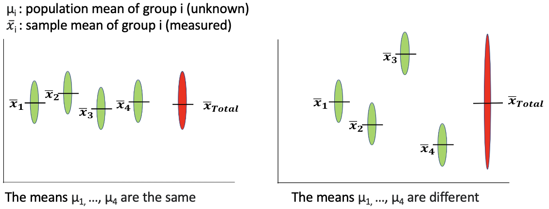
(Figure credit: Lorette Noiret)

  • \(H_0: \mu_1 = \mu_2 = ... = \mu_n\)
  • \(H_1\): there is at least one group which has an average different than other groups.

Which is equals to test:

  • \(H_0: \sigma^2_{\text{inter group}} = \sigma^2_{\text{intra group}}\)
  • \(H_1: \sigma^2_{\text{inter group}} > \sigma^2_{\text{intra group}}\)

If the means are truly different, the variation between groups (\(\sigma^2_{\text{inter group}}\)) should be greater than the variation within groups (\(\sigma^2_{\text{intra group}}\)).

ANOVA calculates the F statistic, which is a ratio:

\(F = \frac{\sigma^2_{\text{inter group}}}{\sigma^2_{\text{intra group}}}\)

, and the probability of obtaining an F-statistic as extreme as the observed one (the p-value), assuming the null hypothesis is true.

Conditions of applying ANOVA:

  • Independence: Observations in each group must be independent.
  • Normality: Data should be approximately normally distributed (can be checked using the Shapiro test).
  • Homoscedasticity (homogeneity of variance): Variances across groups should be roughly equal (Levene’s test or Bartlett’s test can check this).

In R, the function aov() is used to perform ANOVA.

Let’s take the gene LOH1 as example.

  1. Import the expression data using this link: "https://inforbio.github.io/IOC/ioc_r/exos_data/read-counts.csv"
counts <- read_csv(
  "https://inforbio.github.io/IOC/ioc_r/exos_data/read-counts.csv"
)
Rows: 45 Columns: 41
── Column specification ────────────────────────────────────────────────────────
Delimiter: ","
chr  (1): Feature
dbl (40): WT.1, WT.2, WT.3, WT.4, WT.5, WT.6, WT.7, WT.8, WT.9, WT.10, SET1....

ℹ Use `spec()` to retrieve the full column specification for this data.
ℹ Specify the column types or set `show_col_types = FALSE` to quiet this message.
  1. Given the imported counts data, how can we reshape it to extract the necessary information and obtain a tibble with the following columns?
  • “value”: Expression values of the gene LOH1
  • “group”: Sample groups (Explore how to use the str_replace() function to extract group based on sample name)
?str_replace

anova_data <- counts |>
  filter(Feature == "LOH1") |>
  pivot_longer(
    cols = -1,
    names_to = "sample_id",
    values_to = "value"
  ) |>
  mutate(
    group = str_replace(
      string = sample_id,
      pattern = "\\.([0-9]+)$",
      replace = ""
    )
  )
anova_data
# A tibble: 40 × 4
   Feature sample_id value group
   <chr>   <chr>     <dbl> <chr>
 1 LOH1    WT.1         10 WT   
 2 LOH1    WT.2          2 WT   
 3 LOH1    WT.3         14 WT   
 4 LOH1    WT.4         19 WT   
 5 LOH1    WT.5         35 WT   
 6 LOH1    WT.6         17 WT   
 7 LOH1    WT.7          6 WT   
 8 LOH1    WT.8          3 WT   
 9 LOH1    WT.9         31 WT   
10 LOH1    WT.10        13 WT   
# ℹ 30 more rows
  1. Assume that all conditions of ANOVA are verified. Perform an ANOVA (aov()) test and use summary() to obtain the results. If we take \(\alpha=0.05\), what is your conclusion?
res_aov <- aov(value ~ group, data = anova_data)
summary(res_aov)
            Df Sum Sq Mean Sq F value  Pr(>F)    
group        3  45166   15055   13.69 4.1e-06 ***
Residuals   36  39603    1100                    
---
Signif. codes:  0 '***' 0.001 '**' 0.01 '*' 0.05 '.' 0.1 ' ' 1
  1. Conduct a Tukey Honest Significant Differences (TukeyHSD) test to check which groups differ significantly. (?TukeyHSD)
TukeyHSD(res_aov)
  Tukey multiple comparisons of means
    95% family-wise confidence level

Fit: aov(formula = value ~ group, data = anova_data)

$group
                diff        lwr        upr     p adj
SET1-RRP6       62.1   22.15167 102.048326 0.0009619
SET1.RRP6-RRP6   7.7  -32.24833  47.648326 0.9539581
WT-RRP6        -31.2  -71.14833   8.748326 0.1713841
SET1.RRP6-SET1 -54.4  -94.34833 -14.451674 0.0041844
WT-SET1        -93.3 -133.24833 -53.351674 0.0000017
WT-SET1.RRP6   -38.9  -78.84833   1.048326 0.0587008
  1. Visualize the expression levels of the LOH1 gene across the four groups using a boxplot.
ggplot(
  anova_data,
  aes(
    x = factor(group, levels = c("WT", "SET1", "SET1.RRP6", "RRP6")),
    y = value
  )
) +
  geom_boxplot(
    outliers = FALSE # do not display outliers by boxplot
  ) +
  geom_point(
    aes(color = group),
    position = position_jitter(height = 0, width = 0.3, seed = 1)
  ) +
  labs(x = NULL, title = "Expression of LOH1") +
  theme_light() +
  theme(legend.position = "none")

Bonus

Verify the assumptions for conducting an ANOVA test:

# Check data normality with Shapiro test
shapiro.test(anova_data$value[anova_data$group == "WT"])

    Shapiro-Wilk normality test

data:  anova_data$value[anova_data$group == "WT"]
W = 0.92104, p-value = 0.3657
shapiro.test(anova_data$value[anova_data$group == "SET1"])

    Shapiro-Wilk normality test

data:  anova_data$value[anova_data$group == "SET1"]
W = 0.90683, p-value = 0.2599
shapiro.test(anova_data$value[anova_data$group == "SET1.RRP6"])

    Shapiro-Wilk normality test

data:  anova_data$value[anova_data$group == "SET1.RRP6"]
W = 0.92342, p-value = 0.3864
shapiro.test(anova_data$value[anova_data$group == "RRP6"])

    Shapiro-Wilk normality test

data:  anova_data$value[anova_data$group == "RRP6"]
W = 0.81775, p-value = 0.02381
# or use lapply() to repeat test for each group
# lapply(
#   X = unique(anova_data$group),
#   FUN = function(grp) {
#     shapiro.test(anova_data$value[anova_data$group == grp])
#   }
# )

The RRP6 data does not follow a normal distribution.

# Check homogeneity of variance with Bartlett test
bartlett.test(value ~ group, data = anova_data)

    Bartlett test of homogeneity of variances

data:  value by group
Bartlett's K-squared = 25.242, df = 3, p-value = 1.374e-05

Moreover, the assumption of homoscedasticity (equal variance) is not met.

Therefore, an ANOVA is not appropriate, and a non-parametric Kruskal-Wallis test should be used instead.

kruskal.test(value ~ group, data = anova_data)

    Kruskal-Wallis rank sum test

data:  value by group
Kruskal-Wallis chi-squared = 24.631, df = 3, p-value = 1.845e-05

Great work, you’ve made it to the end! 🎉 and now you’re ready to take on even more! Keep exploring new things, there’s so much more R can do for you!