Week 7 - Hands-On Examples

week07
exercise

The R script is available here: link

Goals

  • Use apply() for column-wise and row-wise operations (e.g., calculation variance of each rows or columns)
  • Leverage lapply() for list-based computations (e.g., repeating generation of plot for a list of genes)

The apply() Function

  1. Import the gene expression data file (read-counts.csv) into RStudio and name it as counts.
counts <- read.csv("../exos_data/read-counts.csv", header = TRUE)
dim(counts)
[1] 45 41
counts[1:5, 1:5]
  Feature  WT.1 WT.2 WT.3  WT.4
1    HTB2 20648  466 1783 25335
2    HHF1  7867  147  427  5178
3    HHT1  1481   37  187  1856
4   POL30   743   27  370  4050
5    KCC4   185    6  200   669
  1. Calculate following metrics for each row (genes) and column (samples) using the apply() function:
  • Mean (mean())
  • Variance (var())
  • Minimum and maximum (min(), max() or use range())

What is the expected length or dimension of the outputs?

Attention: exclude the 1st column for the calculation.

## for rows
apply(X = counts[, -1], MARGIN = 1, FUN = var)
 [1] 4.229507e+08 3.264981e+08 5.093724e+06 6.098649e+06 3.167363e+05
 [6] 1.696711e+06 6.243013e+01 5.135088e+07 4.481458e+05 5.613792e+06
[11] 2.828137e+06 3.958020e+03 8.141026e+00 7.387680e+06 9.717232e+04
[16] 1.836038e+04 7.641206e+05 1.215755e+04 2.046040e+07 6.234914e+04
[21] 2.173567e+03 1.323384e+06 1.458099e+05 2.328199e+05 2.355261e+04
[26] 1.484697e+06 3.725897e+01 1.459757e+06 1.020769e+03 2.372274e+06
[31] 5.467048e+05 8.673079e+08 8.258462e+05 1.109506e+06 5.906558e+05
[36] 9.570327e+07 1.357117e+08 5.456164e+04 5.101182e+04 9.259533e+04
[41] 1.144050e+06 4.732471e+05 1.387217e+05 6.364334e+04 2.112346e+04
apply(counts[, -1], 1, mean)
 [1] 27057.100 19500.075  2841.175  2567.275   698.925  1476.225    19.075
 [8]  9192.675   629.550  5955.250  1763.425    77.925     2.750  5930.425
[15]   410.300   144.775  1011.275   155.125  3516.650   330.200    55.850
[22]   696.275   542.025   855.550   310.400  2779.650     7.850  2336.175
[29]    48.000  1981.825  1000.175 27188.625  2231.650  2142.075   959.650
[36] 13984.950 15551.650   358.275   335.650   323.475  1425.650  1546.375
[43]   704.875   319.125   249.850
apply(counts[, -1], 1, min)
 [1] 466 147  37  27   6  16   0 105   8 490  35   0   0 155   8   0  12   4 352
[20]   9   2  40  26  92  43 474   0 527   2  27  10 417 110  45   6 222 136   1
[39]  41   0  42  92  39  10   9
apply(counts[, -1], 1, max)
 [1]  77043  79181   9389  10529   2193   5007     34  26690   2207  11390
[11]   7483    249     11  13542   1222    537   3420    509  23695    924
[21]    203   6014   1472   2210    793   5576     26   5774    123   5935
[31]   2716 143592   5104   5149   2855  43987  48131    823   1134   1281
[41]   4546   3327   1541   1013    617
apply(counts[, -1], 1, range)
      [,1]  [,2] [,3]  [,4] [,5] [,6] [,7]  [,8] [,9] [,10] [,11] [,12] [,13]
[1,]   466   147   37    27    6   16    0   105    8   490    35     0     0
[2,] 77043 79181 9389 10529 2193 5007   34 26690 2207 11390  7483   249    11
     [,14] [,15] [,16] [,17] [,18] [,19] [,20] [,21] [,22] [,23] [,24] [,25]
[1,]   155     8     0    12     4   352     9     2    40    26    92    43
[2,] 13542  1222   537  3420   509 23695   924   203  6014  1472  2210   793
     [,26] [,27] [,28] [,29] [,30] [,31]  [,32] [,33] [,34] [,35] [,36] [,37]
[1,]   474     0   527     2    27    10    417   110    45     6   222   136
[2,]  5576    26  5774   123  5935  2716 143592  5104  5149  2855 43987 48131
     [,38] [,39] [,40] [,41] [,42] [,43] [,44] [,45]
[1,]     1    41     0    42    92    39    10     9
[2,]   823  1134  1281  4546  3327  1541  1013   617
## for columns
apply(X = counts[, -1], MARGIN = 2, FUN = var)
        WT.1         WT.2         WT.3         WT.4         WT.5         WT.6 
  17911055.8     154280.4     994368.1  211585645.4  134241685.1   18814008.3 
        WT.7         WT.8         WT.9        WT.10       SET1.1       SET1.2 
   4497893.3   67829535.7  222471568.1   32253049.4   20529323.0    7290729.0 
      SET1.3       SET1.4       SET1.5       SET1.6       SET1.7       SET1.8 
   2076054.6  568294955.7   81916242.9   15177583.3    4633361.6  152452583.5 
      SET1.9      SET1.10  SET1.RRP6.1  SET1.RRP6.2  SET1.RRP6.3  SET1.RRP6.4 
 172597353.6   74198430.8   78164538.5    3970588.2    1696609.5   74761622.5 
 SET1.RRP6.5  SET1.RRP6.6  SET1.RRP6.7  SET1.RRP6.8  SET1.RRP6.9 SET1.RRP6.10 
 172447809.5   76318703.6   10449234.9    4723211.9   49172763.2   48225365.4 
      RRP6.1       RRP6.2       RRP6.3       RRP6.4       RRP6.5       RRP6.6 
  69513408.2   14784643.0    1131604.1  107500765.2  179151356.9   60363425.4 
      RRP6.7       RRP6.8       RRP6.9      RRP6.10 
  25857006.9   25251454.2  136843124.2  367401358.3 
apply(counts[, -1], 2, mean)
        WT.1         WT.2         WT.3         WT.4         WT.5         WT.6 
    2028.289      148.000      620.600     4304.111     4837.400     2227.089 
        WT.7         WT.8         WT.9        WT.10       SET1.1       SET1.2 
    1385.311     3106.422     6335.178     2770.111     2168.689     1552.956 
      SET1.3       SET1.4       SET1.5       SET1.6       SET1.7       SET1.8 
    1028.622     8848.133     4179.378     2518.578     1566.378     5119.422 
      SET1.9      SET1.10  SET1.RRP6.1  SET1.RRP6.2  SET1.RRP6.3  SET1.RRP6.4 
    5741.089     4421.200     4797.289     1169.356     1152.689     4658.000 
 SET1.RRP6.5  SET1.RRP6.6  SET1.RRP6.7  SET1.RRP6.8  SET1.RRP6.9 SET1.RRP6.10 
    6163.822     4438.089     2011.644     1699.822     4688.889     3627.933 
      RRP6.1       RRP6.2       RRP6.3       RRP6.4       RRP6.5       RRP6.6 
    4280.689     1842.067     1009.889     4954.844     5977.178     3795.378 
      RRP6.7       RRP6.8       RRP6.9      RRP6.10 
    3119.422     3706.978     6139.156     9162.867 
apply(counts[, -1], 2, min)
        WT.1         WT.2         WT.3         WT.4         WT.5         WT.6 
           0            0            0            0            1            0 
        WT.7         WT.8         WT.9        WT.10       SET1.1       SET1.2 
           0            0            2            2            0            0 
      SET1.3       SET1.4       SET1.5       SET1.6       SET1.7       SET1.8 
           1            0            1            0            0            1 
      SET1.9      SET1.10  SET1.RRP6.1  SET1.RRP6.2  SET1.RRP6.3  SET1.RRP6.4 
           1            3            2            5            2            5 
 SET1.RRP6.5  SET1.RRP6.6  SET1.RRP6.7  SET1.RRP6.8  SET1.RRP6.9 SET1.RRP6.10 
           1            3            5            5            9            4 
      RRP6.1       RRP6.2       RRP6.3       RRP6.4       RRP6.5       RRP6.6 
          11            4            1            5            2            4 
      RRP6.7       RRP6.8       RRP6.9      RRP6.10 
           8            5            1            6 
apply(counts[, -1], 2, max)
        WT.1         WT.2         WT.3         WT.4         WT.5         WT.6 
       20648         2527         4242        95501        64252        24126 
        WT.7         WT.8         WT.9        WT.10       SET1.1       SET1.2 
        9067        52051        67353        28059        21214        15057 
      SET1.3       SET1.4       SET1.5       SET1.6       SET1.7       SET1.8 
        6328       143592        39073        17421         9220        76434 
      SET1.9      SET1.10  SET1.RRP6.1  SET1.RRP6.2  SET1.RRP6.3  SET1.RRP6.4 
       56156        42195        36236        11869         6511        44611 
 SET1.RRP6.5  SET1.RRP6.6  SET1.RRP6.7  SET1.RRP6.8  SET1.RRP6.9 SET1.RRP6.10 
       53296        35468        12523         7170        25922        24745 
      RRP6.1       RRP6.2       RRP6.3       RRP6.4       RRP6.5       RRP6.6 
       38560        23695         4076        55657        57599        37863 
      RRP6.7       RRP6.8       RRP6.9      RRP6.10 
       25900        21179        43620        79181 
apply(counts[, -1], 2, range)
      WT.1 WT.2 WT.3  WT.4  WT.5  WT.6 WT.7  WT.8  WT.9 WT.10 SET1.1 SET1.2
[1,]     0    0    0     0     1     0    0     0     2     2      0      0
[2,] 20648 2527 4242 95501 64252 24126 9067 52051 67353 28059  21214  15057
     SET1.3 SET1.4 SET1.5 SET1.6 SET1.7 SET1.8 SET1.9 SET1.10 SET1.RRP6.1
[1,]      1      0      1      0      0      1      1       3           2
[2,]   6328 143592  39073  17421   9220  76434  56156   42195       36236
     SET1.RRP6.2 SET1.RRP6.3 SET1.RRP6.4 SET1.RRP6.5 SET1.RRP6.6 SET1.RRP6.7
[1,]           5           2           5           1           3           5
[2,]       11869        6511       44611       53296       35468       12523
     SET1.RRP6.8 SET1.RRP6.9 SET1.RRP6.10 RRP6.1 RRP6.2 RRP6.3 RRP6.4 RRP6.5
[1,]           5           9            4     11      4      1      5      2
[2,]        7170       25922        24745  38560  23695   4076  55657  57599
     RRP6.6 RRP6.7 RRP6.8 RRP6.9 RRP6.10
[1,]      4      8      5      1       6
[2,]  37863  25900  21179  43620   79181

The lapply() Function

Check GC Content

The GC content is the percentage of guanine (G) and cytosine (C) in a DNA or RNA sequence. This measure is one of the metrics which can be used in the sequencing quality control (e.g., detects contamination).

Here we will use a small example to see how this metric is calculated.

# Generate a list of DNA sequences
dna_sequences <- list(
  seq1 = "ATGCGTAGCTAGGCTATCCGA",
  seq2 = "CGCGTTAGGCAAGTGTTACG",
  seq3 = "GGTACGATCGATGCGCGTAA",
  seq4 = "TTTAAACCCGGGATATAAAA"
)

# the 1st DNA sequence
dna_sequences[["seq1"]]
[1] "ATGCGTAGCTAGGCTATCCGA"
  1. Split the 1st DNA sequence into individual bases using the function strsplit(). (See ?strsplit)
seq1 <- strsplit(dna_sequences[["seq1"]], split = "")
seq1
[[1]]
 [1] "A" "T" "G" "C" "G" "T" "A" "G" "C" "T" "A" "G" "G" "C" "T" "A" "T" "C" "C"
[20] "G" "A"
  1. Convert the results of split to a vector.
seq1_base <- unlist(seq1)
seq1_base
 [1] "A" "T" "G" "C" "G" "T" "A" "G" "C" "T" "A" "G" "G" "C" "T" "A" "T" "C" "C"
[20] "G" "A"
  1. Count the number of G and C bases among all bases.
seq1_base %in% c("G", "C")
 [1] FALSE FALSE  TRUE  TRUE  TRUE FALSE FALSE  TRUE  TRUE FALSE FALSE  TRUE
[13]  TRUE  TRUE FALSE FALSE FALSE  TRUE  TRUE  TRUE FALSE
gc_count <- sum(seq1_base %in% c("G", "C"))
gc_count
[1] 11
  1. Calculate the percentage of GC in the whole sequence.
gc_percentage <- gc_count / length(seq1_base) * 100
gc_percentage
[1] 52.38095
  1. Write a function which take one sequence as input to calculate the GC content. Test your function on the 1st sequence of the list.
# Function to calculate GC content
gc_content <- function(sequence) {
  seq_base <- unlist(strsplit(sequence, ""))  # Split sequence into individual bases
  gc_count <- sum(seq_base %in% c("G", "C"))  # Count G and C bases
  gc_percentage <- (gc_count / length(seq_base)) * 100  # Calculate percentage
  return(gc_percentage)
}

gc_content(dna_sequences[["seq1"]])
[1] 52.38095
  1. Use lapply() or sapply() to apply the created function to the list of sequences.
# Apply function to all sequences
lapply(dna_sequences, gc_content)
$seq1
[1] 52.38095

$seq2
[1] 55

$seq3
[1] 55

$seq4
[1] 30
sapply(dna_sequences, gc_content)
    seq1     seq2     seq3     seq4 
52.38095 55.00000 55.00000 30.00000 

Automate Tasks for a List of Genes

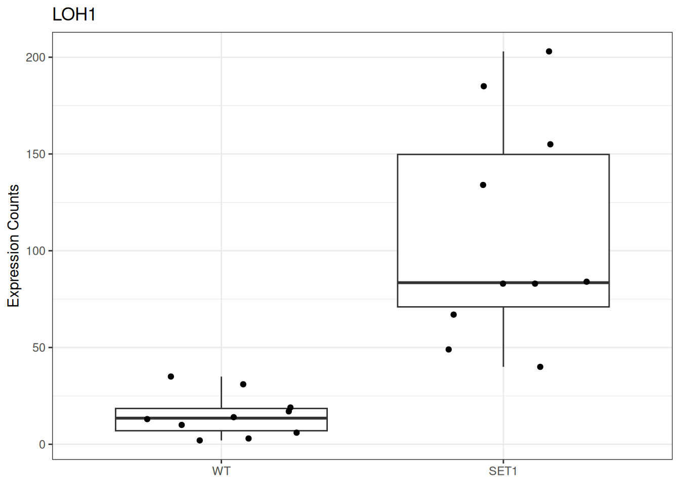
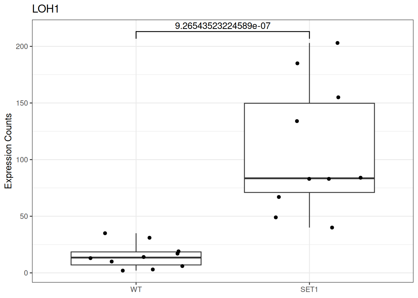
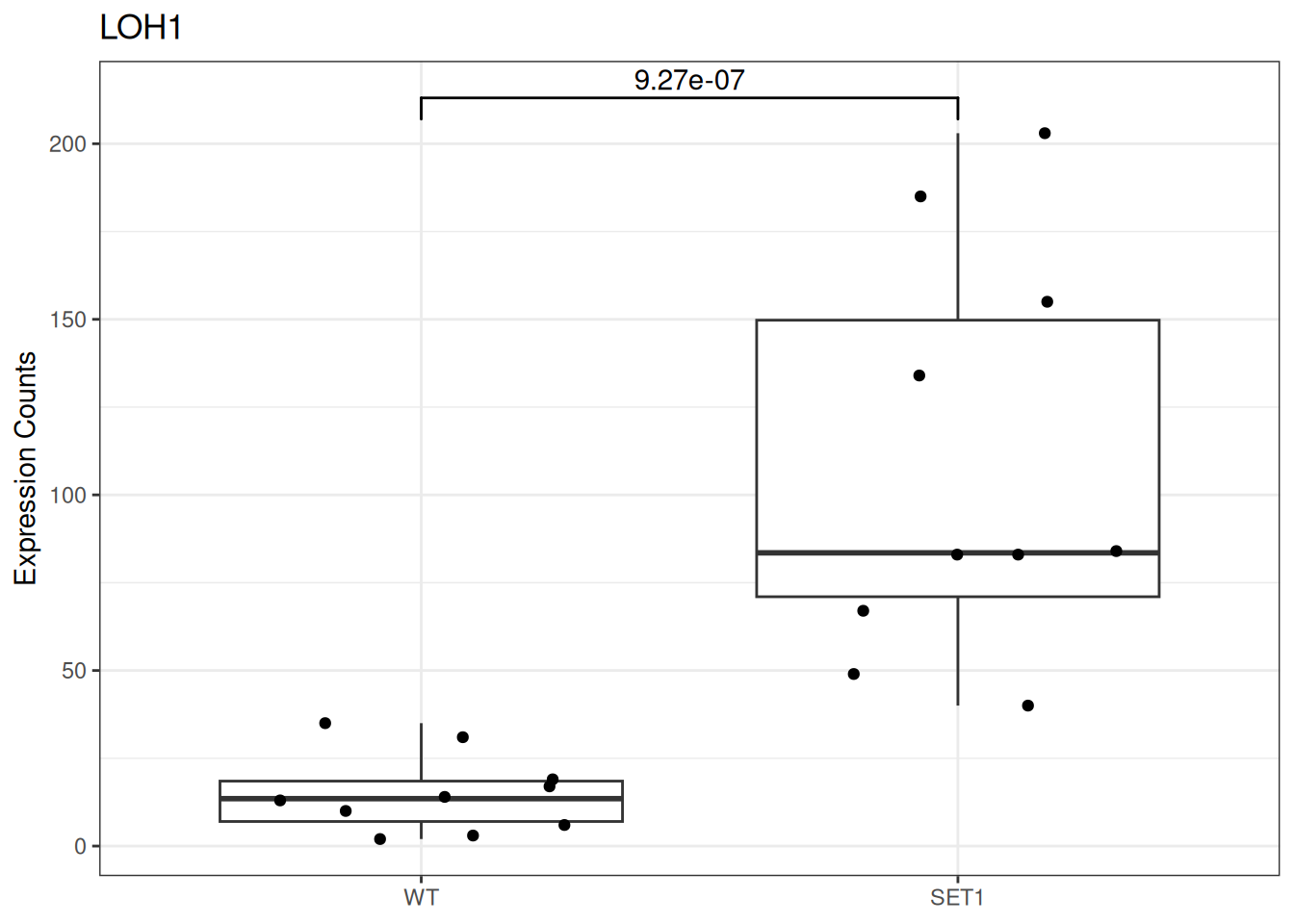
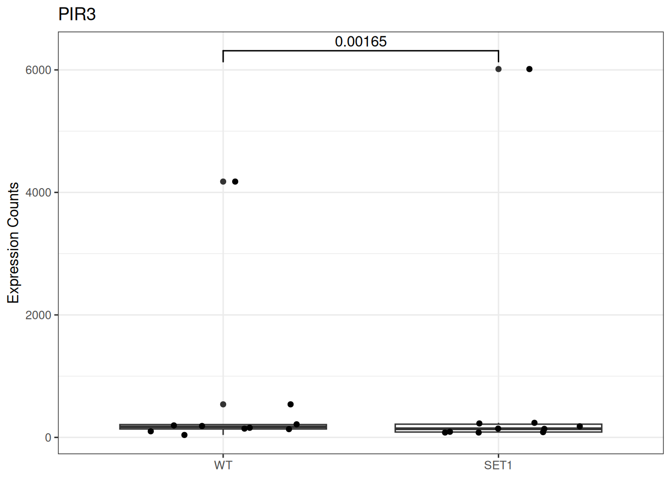
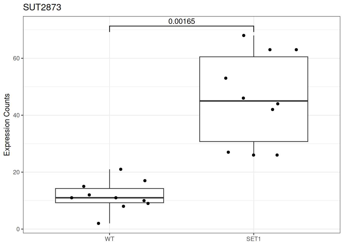
Based on differential gene expression analysis (SET1 vs. WT) results, draw the boxplot of for the top 3 genes with the smallest adjusted p-value, add individual data points on the boxplot and show p-value above the boxes with horizontal bar (with the help of the {ggsignif} pacakge).

  1. Import the differential gene expression analysis (SET1 vs. WT) results file toy_DEanalysis.csv into RStudio and name it as de_res.
# Import DE results
de_res <- read.csv("../exos_data/toy_DEanalysis.csv", header = TRUE)
head(de_res)
  gene_name   baseMean log2FoldChange     lfcSE       stat    pvalue      padj
1      HTB2 20259.4339    -0.37571144 0.4468852 -0.8407337 0.4004971 0.8912909
2      HHF1  9820.5151     0.17885040 0.5357945  0.3338041 0.7385274 0.9062761
3      HHT1  1538.5211     0.08662417 0.4124190  0.2100392 0.8336371 0.9149675
4     POL30  1273.9493     0.41649987 0.4215451  0.9880316 0.3231372 0.8912909
5      KCC4   315.6121     0.21894618 0.4337310  0.5047972 0.6137013 0.8912909
6      MCD1   632.4889     0.21098855 0.3645113  0.5788258 0.5627067 0.8912909
  1. Extract the genes of interest, i.e., 3 genes with the smallest adjusted p-value.
# Order data by adjusted pvalue
de_res <- de_res[order(de_res$padj), ]
head(de_res)
   gene_name   baseMean log2FoldChange     lfcSE      stat       pvalue
21      LOH1   48.61440      2.2259655 0.3969997  5.606971 2.058986e-08
22      PIR3  304.29450     -2.3659253 0.6082583 -3.889672 1.003798e-04
29   SUT2873   26.00372      1.4253323 0.3685458  3.867449 1.099797e-04
9     SUT476   88.12355      0.9935943 0.3856808  2.576209 9.989029e-03
10     APQ12 5422.70915     -0.6401330 0.2366950 -2.704463 6.841488e-03
20     SUT24  155.78840     -0.8436243 0.3281685 -2.570705 1.014917e-02
           padj
21 9.265435e-07
22 1.649695e-03
29 1.649695e-03
9  7.611881e-02
10 7.611881e-02
20 7.611881e-02
# Extract the first 3 gene names
target_genes <- de_res[1:3, "gene_name"]
target_genes
[1] "LOH1"    "PIR3"    "SUT2873"
# alternatives
# target_genes <- de_res[order(de_res$padj), ][1:3, "gene_name"]
# target_genes <- de_res[order(de_res$padj), ]$gene_name[1:3]
  1. Based on the counts data, build data frame for the LOH1 gene for the boxplot. This data frame should contain:
  • a column of counts for SET1 and WT samples,
  • and a column for corresponding the sample group.

Attention: In order to avoid hardcoding the gene name or sample name, use a variable instead.

# create a variable to store gene name
my_gene <- "LOH1"
# even better
my_gene <- target_genes[1]

# create another variable for the number of sample
1:10 # old way
 [1]  1  2  3  4  5  6  7  8  9 10
n_sample <- 10
seq(n_sample)
 [1]  1  2  3  4  5  6  7  8  9 10
seq_len(n_sample) # safer, take only non negative number
 [1]  1  2  3  4  5  6  7  8  9 10
gg_df <- data.frame(
  expr_val = c(
    unlist(counts[counts$Feature == my_gene, paste0("WT.", seq_len(n_sample))]),
    unlist(counts[counts$Feature == my_gene, paste0("SET1.", seq_len(n_sample))])
  ),
  group = factor(
    rep(c("WT", "SET1"), each = n_sample),
    levels = c("WT", "SET1")
  )
)
head(gg_df)
     expr_val group
WT.1       10    WT
WT.2        2    WT
WT.3       14    WT
WT.4       19    WT
WT.5       35    WT
WT.6       17    WT
## alternative
# gg_df <- as.data.frame(t(
#   counts[
#     counts$Feature == my_gene,
#     paste0(
#       rep(c("WT.", "SET1."), each = n_sample),
#       seq_len(n_sample)
#     )
#   ]
# ))
# colnames(gg_df) <- "expr_val"
# gg_df$group <- factor(rep(c("WT", "SET1"), each = n_sample), levels = c("WT", "SET1"))
## or
# gg_df <- data.frame(
#   expr_val = unlist(
#     counts[
#       counts$Feature == my_gene,
#       paste0(
#         rep(c("WT.", "SET1."), each = n_sample),
#         seq_len(n_sample)
#       )
#     ]
#   ),
#   group = factor(
#     rep(c("WT", "SET1"), each = n_sample),
#     levels = c("WT", "SET1")
#   )
# )
  1. Draw boxplot and show the individual data points on the same figure.
library(ggplot2)

p <- ggplot(gg_df, aes(x = group, y = expr_val)) +
  geom_boxplot() +
  geom_point(
    position = position_jitter(width = 0.3, height = 0, seed = 1)
  ) +
  labs(x = NULL, y = "Expression Counts", title = my_gene) +
  theme_bw()

p

  1. Add p-value with a horizontal bar on the figure:
  • install the ggsignif package,
  • use the function geom_signif() to add a layer to show p-value on the figure.

Check the documentation of geom_signif(), what do we need to add p-value?

# install.packages("ggsignif")
library(ggsignif)

p + geom_signif(
  comparisons = list(c("WT", "SET1")),
  annotations = de_res$padj[de_res$gene_name == my_gene] # show p-value as is
)

# improve p-value annotation
p <- p + geom_signif(
  comparisons = list(c("WT", "SET1")),
  annotations = signif( # round p-value
    de_res$padj[de_res$gene_name == my_gene],
    digits = 3
  )
)

p

  1. Generalise previous steps with a function which take the name of gene as input. Test the function with another gene.
draw_boxplot <- function(gene_i) {
  ## build data frame for the plot
  gg_df <- data.frame(
    expr_val = c(
      unlist(counts[counts$Feature == gene_i, paste0("WT.", 1:10)]),
      unlist(counts[counts$Feature == gene_i, paste0("SET1.", 1:10)])
    ),
    group = factor(rep(c("WT", "SET1"), each = 10), levels = c("WT", "SET1"))
  )

  ## draw figure
  p <- ggplot(gg_df, aes(x = group, y = expr_val)) +
    geom_boxplot() +
    geom_point(
      position = position_jitter(width = 0.3, height = 0, seed = 1)
    ) +
    labs(x = NULL, y = "Expression Counts", title = gene_i) +
    geom_signif(
      comparisons = list(c("WT", "SET1")),
      annotations = signif(
        de_res$padj[de_res$gene_name == gene_i],
        digits = 3
      )
    ) +
    theme_bw()

  return(p)
}

draw_boxplot(target_genes[2])

  1. Apply the function to the targeted genes.
lapply(target_genes, draw_boxplot)
[[1]]


[[2]]


[[3]]


Good job! 👏👏 You’ve leveled up in R! From basic functions to powerful apply techniques—keep exploring and practicing!