getwd() # show the current working directory

abs_path <- "" # put your answer between quotes
rel_path <- "" # put your answer between quotes

file.exists(abs_path) # check if R finds your file using absolute path
file.exists(rel_path) # check if R finds your file using relative pathWeek 1 - Hands-On Examples
week01
exercise
Goals
- Get familiar with the RStudio
- Create an R project in RStudio
- Import data file into RStudio
- Generate your first Quarto report
Create an R project
- In RStudio, create a new project in your folder.
Some rules for naming your project:
- Choose a short and descriptive name.
- Use snake case (lowercase letters and underscores only). Avoid special characters (such as
!,#, ) and spaces. - The name cannot starts with numbers.
Open your R project, create three new folders, i.e.,
data,scripts,outputs.Download two files:
- An R script named “r_w01_exos.R” for this week’s exercise (here), save it into the
scriptsfolder. - A data file called “read-counts.csv” (here), put it into the
datafolder.
Tip
If you are using RStudio server, files can be uploaded using the “Upload” icon in the Files pane.
Files Description
Data File
We’ll be working with a gene expression dataset as an example, sourced from this link.
The data comes from an experiment using PCR to study 44 genes. The results were measured to see which genes are active at different stages in Yeast cell cycling. Several strains were tested, including wildtype and some with specific genes knock-downs. Samples were taken at nine time points over two cell cycles (two hours).
The R script
The r_w01_exos.R script contains all commands R for the exercise.
Play with RStudio
In your R project, open the downloaded R script r_w01_exos.R: In RStudio menu bar, click File -> Open File -> selec the Rscript, or click the file in the Files pane.
Import Data
- Click on the CSV file in Files pane to “View” it. Identify the column separator.
- Import the file into R and call the imported data “counts”.
- Copy paste the command shown in the R console.
Exercises
- What is the absolute file path of the imported data
counts? What is its relative path? Verify your answer using the functionfile.exists().
- What is the dimension of the data frame? Check the “Environment” panel or use the function
dim().
dim(counts)[1] 45 41In the “Environment” panel, click on the tabular icon next to the dataset to visualize the it.
We can extract all gene expressions for the sample named “WT.2” using counts[["WT.2"]].
- Try
mode()on the expression data for “WT.2”, what does it return?
mode(counts[["WT.2"]])[1] "numeric"- Calculate the average expression (
mean()) and standard deviation (sd()) of genes from the sample “WT.2”.
mean(counts[["WT.2"]])[1] 148sd(counts[["WT.2"]])[1] 392.7854- Generate descriptive statistics for all genes from the sample “WT.2” using
summary().
summary(counts[["WT.2"]]) Min. 1st Qu. Median Mean 3rd Qu. Max.
0 6 27 148 110 2527
Stats Time!
What are quartiles?
Quartiles are three values that split sorted data into four equal parts.
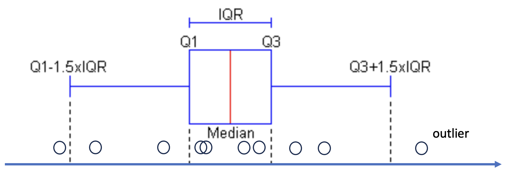
(figure modified from this source)
IQR (Interquartile range) = Q3 - Q1
- Generate a histogram for the “WT.2” sample using
hist(). What does the distribution look like?
Stats Time!
Histograms help us see how data is spread out. They show how many data points fall into different intervals, or bins. By looking at a histogram, we can quickly understand the shape of the data, like if it’s skewed or has outliers. It’s a simple way to get an overview of your data.
hist(counts[["WT.2"]])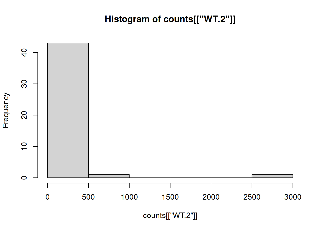
Stats Time!
log2 Transformation
A log2 transformation is commonly used to normalize data and reduce skewness, especially in datasets with values spanning several orders of magnitude. Many biological data, like gene expression counts, tend to have a highly skewed distribution with a long tail of large values. The log2 transformation helps:
- Stabilize variance – Makes data with large differences more comparable.
- Handle ratios – Converts multiplicative relationships into additive ones, simplifying interpretation.
- Improve normality – Makes the data distribution closer to normal, which is often required for statistical tests.
plot(
  x = counts[["WT.2"]], y = log2(counts[["WT.2"]]),
  xlab = "Original Scale", ylab = "log2 Scale",
  main = "Gene expression for the sample WT.2"
)
abline(v = 256, col = "red", lty = 2) # Add vertical line
abline(h = 8, col = "red", lty = 2) # Add horizontal line
text(x = 500, y = 7, labels = expression(2^8 == 256)) # Add equation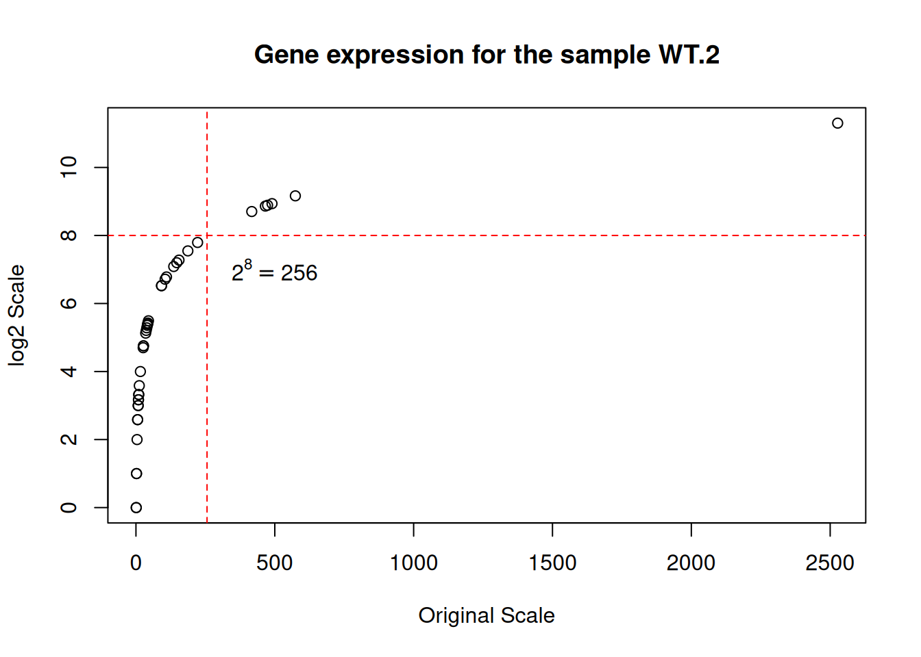
Re draw the histogram with the log2 transformed data, what does the distribution look like now?
hist(log2(counts[["WT.2"]]))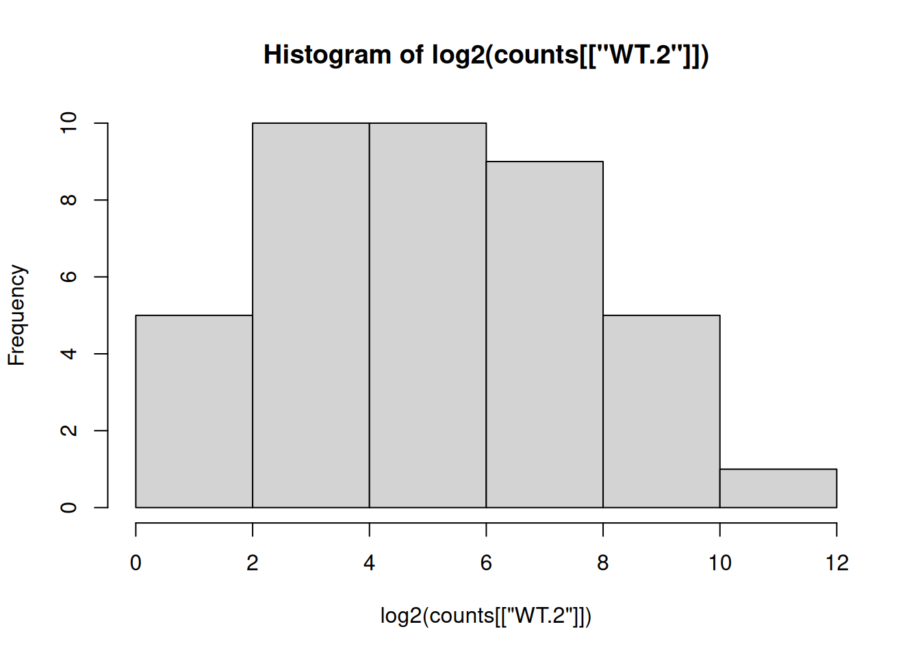
Get Your First Quarto Report
Create a new Quarto document (File -> New File -> Quarto Document), write all codes above and your observation for the questions in the document. Then click the “Render” to generate your own report!
- Change something in your script Quarto and re-render it, is the report up-to-date?
To go further:
- Where is your report stored?
- What should you do if you want the report be stored in a specified folder? => use a configuration file for Quarto.
Open a new text file and copy paste following code, save it as _quarto.yml in your project folder.
project:
  output-dir: outputs/
Try “Render” again, now where is your report?